Amazon Redshift Architecture
Amazon Redshift is a fully managed, massively parallel processing (MPP)
cloud data warehouse. It is designed for analytical workloads such as
reporting, dashboards, and large-scale SQL queries over structured data.
This tutorial explains the main components of Redshift architecture and
how they work together.
High-Level Architecture Overview
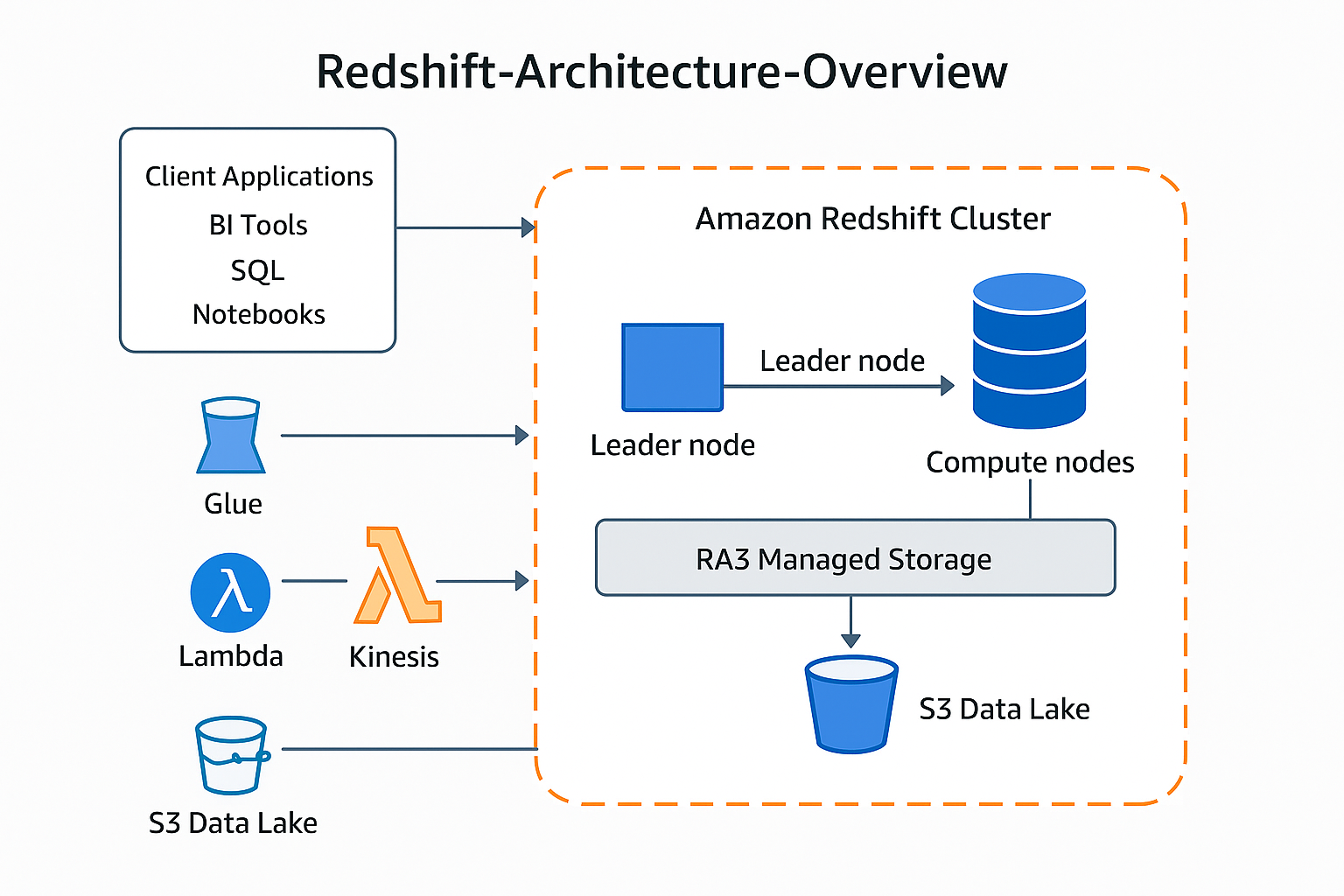
The diagram below summarizes the high-level Amazon Redshift architecture.
-
Client Applications – BI tools, SQL editors, and
notebooks connect to Redshift over JDBC, ODBC, or the Data API.
-
Redshift Cluster – A collection of nodes (one leader
node and one or more compute nodes) that execute queries and store data.
-
Managed Storage and Data Lake – RA3 nodes use managed
storage that can transparently extend into Amazon S3, and Redshift
Spectrum lets you query data directly in S3.
-
Surrounding AWS Services – Services such as S3, Glue,
Lambda, Kinesis, and others integrate for ingestion, cataloging, ETL,
and analytics.
Cluster Components
1. Leader Node
-
Entry point – All client connections terminate at the
leader node.
-
SQL parser and optimizer – Parses incoming SQL, builds
execution plans, and decides how to distribute work across compute
nodes.
-
Coordinator – Sends query fragments to compute nodes
and aggregates the intermediate results.
-
Catalog store – Holds metadata about databases,
schemas, tables, and permissions.
2. Compute Nodes
-
Parallel workers – Each node runs multiple
slices (worker processes). Slices operate on different
portions of the data in parallel.
-
Local storage / cache – Data blocks are stored in
columnar format. RA3 nodes cache frequently used blocks on fast SSD
while automatically managing older blocks in S3.
-
Distribution styles – Data is distributed across nodes
using:
- KEY – rows with the same key go to the same node
- EVEN – rows distributed round-robin
- ALL – small dimension tables fully replicated
-
Columnar storage and compression – Only relevant
columns are read during queries, and compression reduces I/O and cost.
Storage and Data Lake Integration
1. Managed Storage (RA3)
-
Compute and storage decoupled – You can scale compute
capacity (number of nodes) independently from how much data you store.
-
Automatic tiering – Hot data stays in SSD cache; cold
data is transparently moved to Amazon S3.
-
No application changes – From the user’s perspective,
the data behaves like local disk.
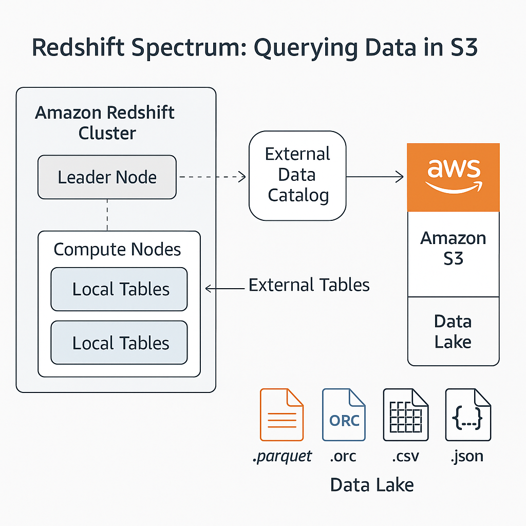
2. Redshift Spectrum: Querying Data in S3
Redshift Spectrum allows you to run queries against structured data stored
directly in Amazon S3, without loading it into local Redshift tables.
-
External tables – Defined in an external data catalog
such as AWS Glue. They reference data files (Parquet, ORC, CSV, JSON)
in S3.
-
Hybrid queries – A single SQL query can join local
Redshift tables with external tables in S3.
-
Pushdown of filters – Projection and filtering are
pushed down to the Spectrum layer to minimize data scanned from S3.
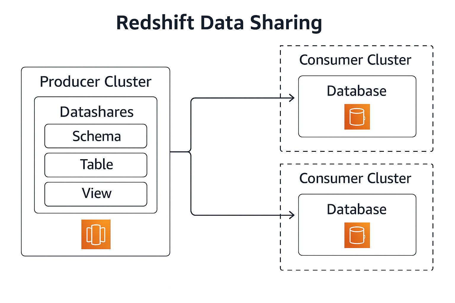
Data Sharing Between Redshift Clusters
Amazon Redshift enables secure data sharing across clusters within the
same AWS account or across accounts. This is useful for sharing curated
data with different business units, teams, or workloads without copying
data.
-
Producer cluster – Owns the physical data and defines
datashares that expose specific schemas, tables, and
views.
-
Consumer clusters – Attach the datashares as standard
database objects and query them as if they were local.
-
No data duplication – Data stays in the producer
cluster’s storage; consumers access it in-place.
-
Fine-grained permissions – Producers control which
objects are shared and who can access them.
Workload Management and Scaling
1. Workload Management (WLM)
-
Queues – Queries are routed into WLM queues, which
define memory allocation and concurrency for different workloads.
-
Automatic WLM – Redshift can automatically manage
memory and concurrency, reducing the need for manual tuning.
-
Query monitoring rules – Rules can log, hop, or abort
queries based on thresholds (runtime, rows scanned, etc.).
2. Concurrency Scaling and Elastic Resize
-
Concurrency Scaling – Redshift automatically adds
transient clusters to absorb short-lived spikes in query load.
-
Elastic resize – Allows you to change the number or
type of nodes for a cluster to handle larger or smaller workloads over
time.
Security and Networking
1. Network Isolation
-
Amazon VPC – Clusters run inside a virtual private
cloud; security groups and network ACLs control inbound and outbound
access.
-
Private connectivity – You can use VPN, Direct Connect,
or VPC peering to securely connect on-premises systems or other VPCs.
2. Encryption and Access Control
-
Encryption at rest – Data can be encrypted using AWS
KMS keys or hardware security modules.
-
Encryption in transit – Connections from clients can be
protected with SSL/TLS.
-
IAM integration – IAM roles grant Redshift permission
to read and write data in S3 for COPY and UNLOAD operations.
-
Database privileges – Users and groups are granted
privileges on schemas, tables, and views, with support for row-level and
column-level security.
Typical Query Lifecycle
-
A client application sends a SQL query to the Redshift
endpoint.
-
The leader node parses, optimizes, and generates a
distributed execution plan.
-
The leader node dispatches work to slices on the
compute nodes.
-
Compute nodes scan columnar data from local or managed
storage and optionally read external data from S3 via Spectrum.
-
Compute nodes aggregate intermediate results and send
them back to the leader node.
-
The leader node performs the final aggregation or sorting
and returns the result set to the client.
Putting It All Together
In practice, a Redshift-based analytics platform typically includes:
-
Data sources – Operational databases, event streams,
and flat files.
-
Ingestion and ETL/ELT – Data is moved into S3 and then
into Redshift using COPY, Glue jobs, Lambda, or third-party ETL tools.
-
Curated warehouse – Dimensional models and fact tables
stored in Redshift and shared with downstream teams using data sharing.
-
Consumption layer – Dashboards, ad-hoc analytics, and
machine-learning workloads running on top of Redshift and S3.
Use the diagrams above together with the section explanations as a visual
tutorial for understanding how Amazon Redshift is structured and how data
flows through the system.
Data Ingestion Pipeline
The Redshift ingestion pipeline represents the flow of data from operational
systems and external data sources into Amazon Redshift. This process typically
involves extraction from sources, transformation into optimized formats, and
loading into Amazon S3 before final ingestion into Redshift.
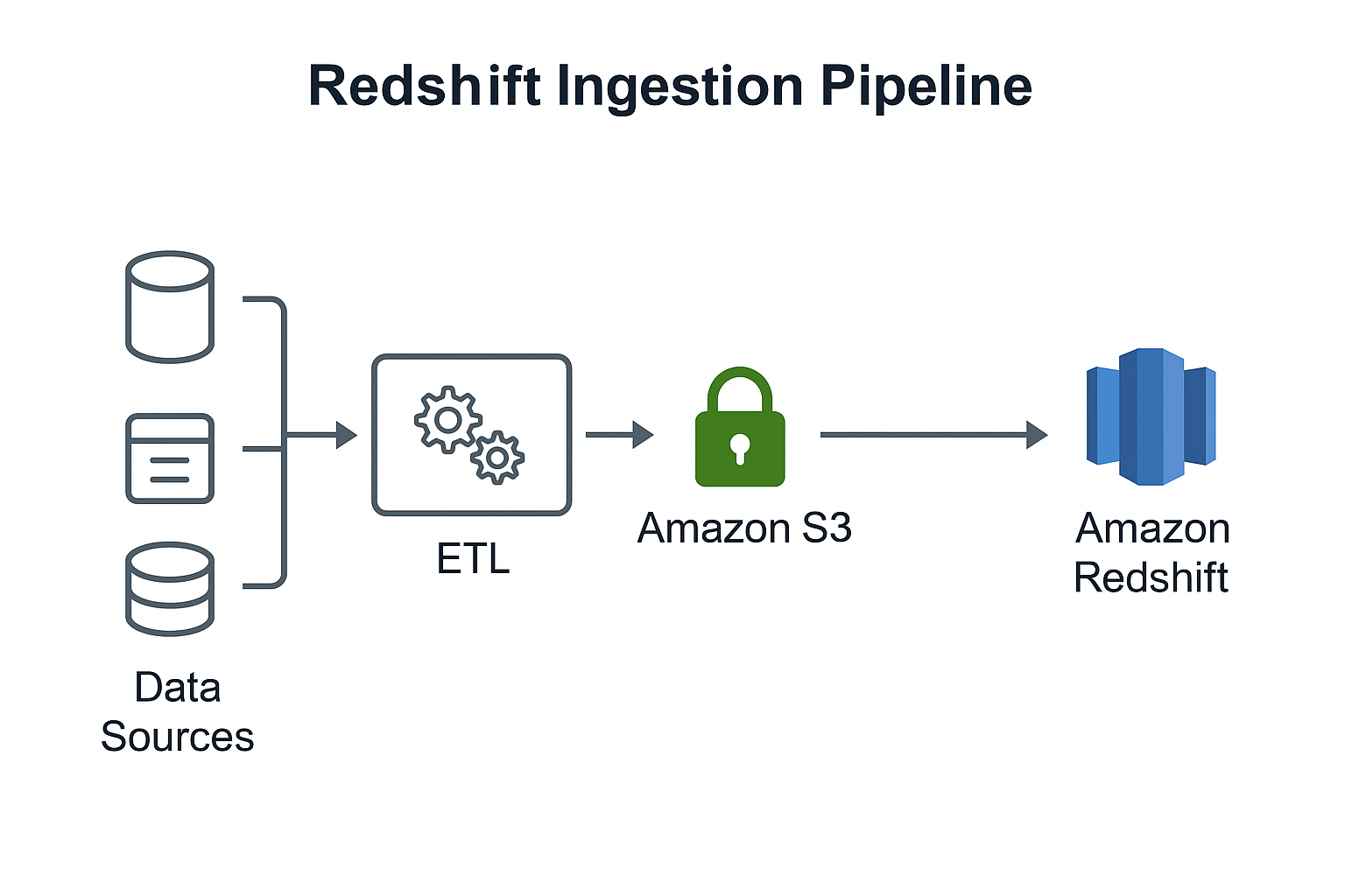
- Data Sources – Operational databases, application logs,
third-party APIs, event streams, and files.
- ETL / ELT Layer – AWS Glue, Lambda, EMR, or third-party
tools perform transformations and cleaning.
- Amazon S3 – The primary ingestion landing zone used for
staging raw and transformed data.
- Amazon Redshift – Final destination for structured
analytics workloads. Data is typically loaded using the COPY command for
maximum throughput.
End-to-End Architecture
The end-to-end Redshift architecture shows the complete lifecycle of data –
from initial collection, through ingestion and transformation, into Amazon
Redshift, and finally consumed by analytics and BI tools.
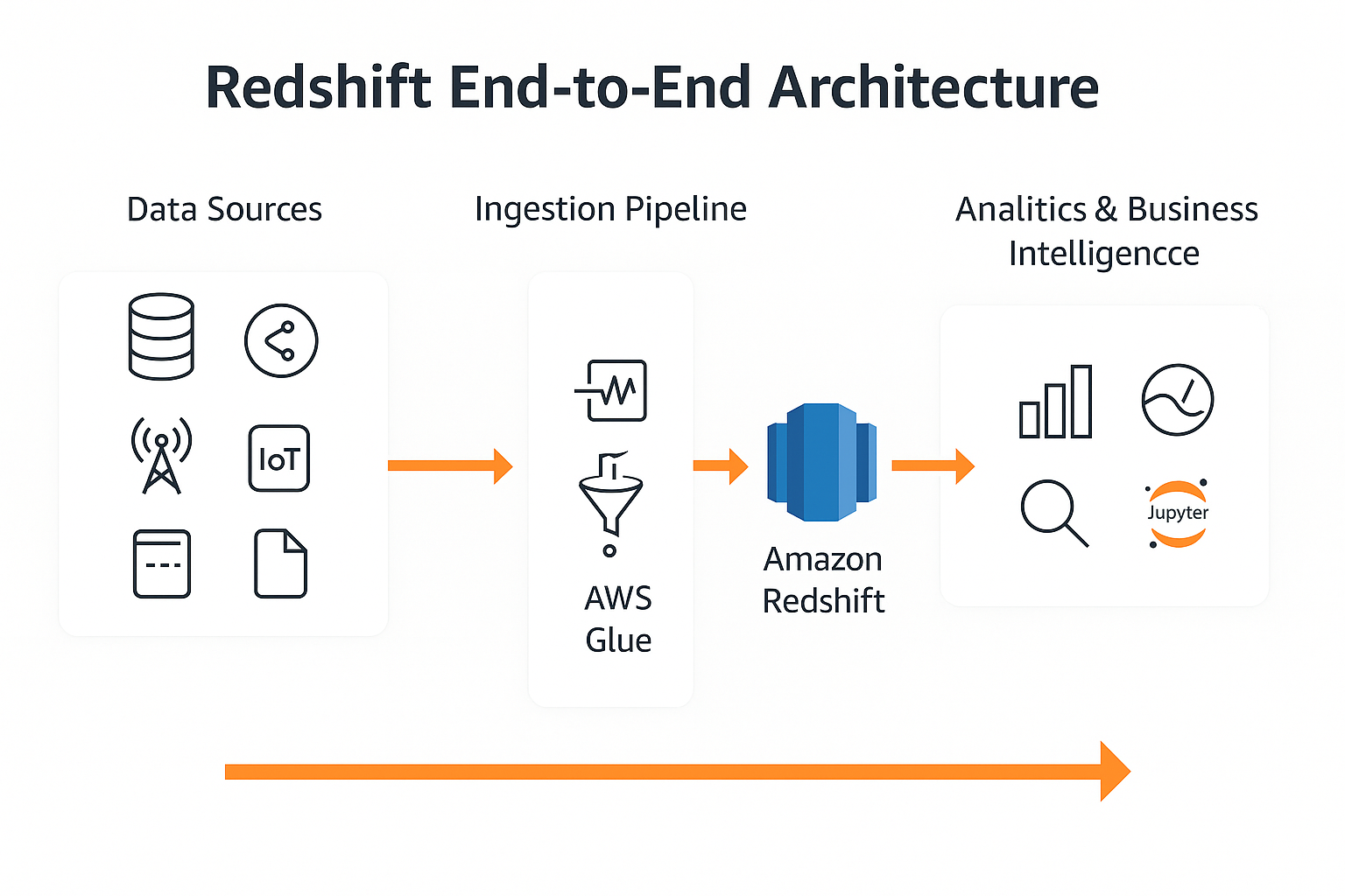
- Data Sources – Databases, applications, IoT, streaming
services, and file-based inputs.
- Ingestion Pipeline – Data flows into S3 or streams
through Kinesis before entering Redshift.
- AWS Glue – Optional transformation stage to clean,
normalize, or enrich data before SQL analytics.
- Amazon Redshift – Central data warehouse storing curated
datasets, fact tables, and dimensional models.
- Analytics & Business Intelligence – Tools such as
QuickSight, Tableau, Looker, and Jupyter notebooks read from Redshift
for dashboards, reporting, and ML workloads.